Linear Quadratic Regulator

Typically, it is challenging to compute value function analytically from the Bellman equation. In fact, we will discuss a variety of methods to approximately obtain the value function later. However, for a certain restricted class of problems, the value function can be obtained in closed form. One such problem is that of the Linear Quadratic Regulator (LQR).

LQR is an optimal control problem that deals with a linear dynamical system and a quadratic cost. Specifically, consider a discrete-time linear dynamical system (for simplicity, we assume a 1-dimensional state and input):

$$\begin{aligned} x_{t+1} & =a x_t+b u_t, t \in\{0,1, \ldots, N\} \tag{1} \\ x_0 & =x^{\text {init }} \end{aligned}$$

Our goal is to minimize a quadratic cost function:

$$J\left(x_0, u_{0: N-1}\right)=\sum_{\tau=0}^{N-1}\left(q x_\tau^2+r u_\tau^2\right)+q_f x_N^2, \tag{2}$$

where $q, r, q_f>0$ are cost penalties. In equation (2):

• $N$ is called the time horizon;
• $q x_\tau^2$ measures state deviation cost at $\tau=t$
• $r u_\tau^2$ measures input authority cost at $\tau=t$
• $q_f x_N^2$ measures the terminal cost.

Thus, we would like to solve the following optimization problem:

$$\min _{u_0: N-1}\left\{J\left(x_0, u_{0: N-1}\right) \text { subject to (1) }\right\} \tag{3}$$

Since the cost is quadratic and dynamics are linear, the above optimal control problem is a convex optimization problem. This convexity allows us to use a variety of optimization tools to solve this problem exactly. In addition, this is one of the optimal control problems, where the optimal control can be obtained in closed form using dynamic programming. These are some of the key reasons for the popularity of LQR in control and robotics literature.

Closed-form Derivation

$$\begin{aligned} J_t^*\left(x_t, u_t\right) & =\min _{u_t}\left\{q x_t^2+r u_t^2+J_{t+1}^*\left(x_{t+1}\right)\right\} \\ & =\min _{u_t}\left\{q x_t^2+r u_t^2+p_{t+1} x_{t+1}^2\right\} . \\ & =\min _{u_t}\left\{q x_t^2+r u_t^2+p_{t+1} a^2 x_t^2+2 p_{t+1} a b x_t u_t+p_{t+1} b^2 u_t^2\right\} \end{aligned}$$

We apply first-order optimality condition $\frac{d J_t^*}{d u_t}=0$

$$\begin{aligned} 2 r u_t+2 p_{t+1} a b x_t+2 p_{t+1} b^2 u_t & =0 \\ u_t^* & =-\frac{p_{t+1} a b x_t}{r+p_{t+1} b^2}=-k_t x_t \\ k_t & =\frac{p_{t+1} a b}{r+p_{t+1} b^2} \end{aligned}$$

$$\begin{aligned} J_t^*\left(x_t\right) & = q x_t^2+r\left(-k_t x_t\right)^2+p_{t+1} a^2 x_t^2+2 p_{t+1} a b x_t\left(-k_t x_t\right) +p_{t+1} b^2\left(-k_t x_t\right)^2 \\ &=\left(q+r k_t^2+p_{t+1} a^2-2 p_{t+1} a b k_t+p_{t+1} b^2 k_t^2\right) x_t^2 \\ &= p_t x_t^2 \\ & \Rightarrow p_t =q+r k_t^2+p_{t+1} a^2-2 p_{t+1} a b k_t+p_{t+1} b^2 k_t^2 \end{aligned}$$

Code Implementation

import matplotlib.pyplot as plt

if __name__ == '__main__':
    a = 1
    b = 1
    q = 1
    qf = q
    r = 1
    N = 20
    x0 = 1
    p_list = [0] * (N + 1)
    k_list = [0] * (N + 1)
    state_list = [0] * (N + 2)
    state_list[0] = x0
    cost_list = [0] * (N + 1)

    # Backward computation for p and k
    def LQR(n):
        if n == N:
            p_list[n] = qf
            return
        else:
            LQR(n + 1)
            k_list[n] = p_list[n + 1] * a * b / (r + p_list[n + 1] * b ** 2)
            p_list[n] = q + r * k_list[n] ** 2 + p_list[n + 1] * a ** 2 - 2 * \
                p_list[n + 1] * a * b * k_list[n] + \
                p_list[n + 1] * b ** 2 * k_list[n] ** 2
        return
    LQR(0)

    # Forward computation for the value function
    for t in range(N + 1):
        cost_list[t] = p_list[t] * state_list[t] ** 2
        u_star = - k_list[t] * state_list[t]
        state_list[t + 1] = a * state_list[t] + b * u_star

    # Compute control
    u_list = []
    for t in range(N + 1):
        u_list.append(-k_list[t] * state_list[t])

    # Plot them
    plt.title("q = " + str(q) + ", r = " + str(r))
    plt.plot(range(N + 1), cost_list, label="cost-to-go")
    plt.plot(range(N + 2), state_list, label="state")
    plt.plot(range(N + 1), u_list, label="control")
    plt.legend()
    plt.show()

Plot

Note

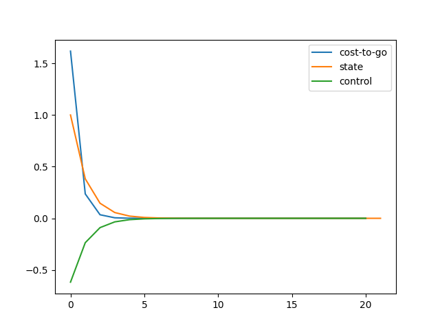
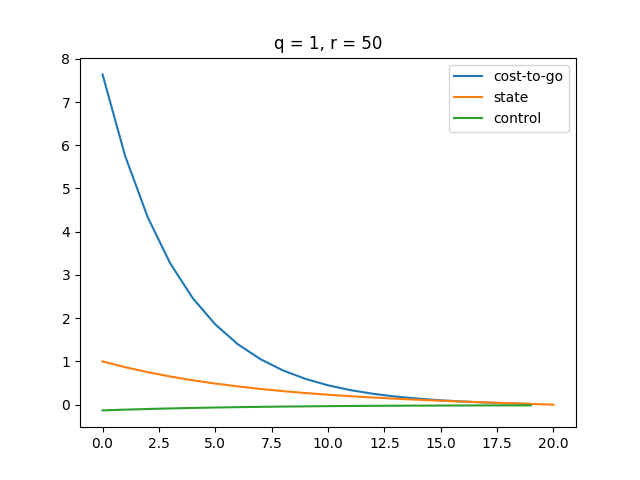
The function approximately converges at around $t=5$.

Behavior Analysis

Note

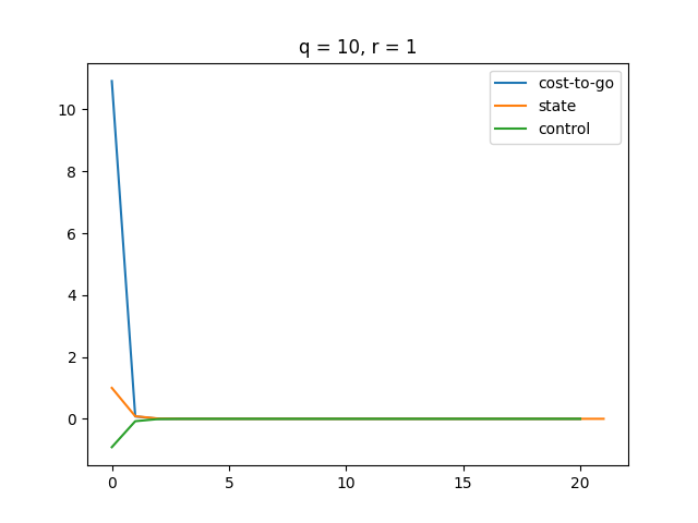
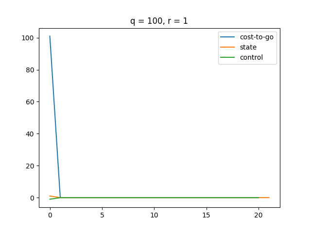
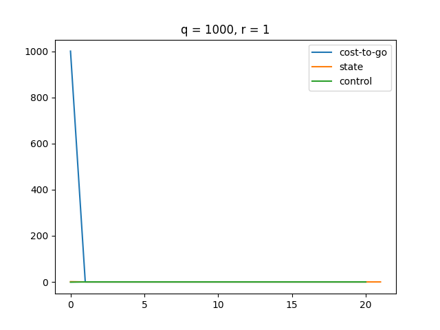
A higher $q$ makes the LQR controller more sensitive to changes in state $x_t$. Thus, LQR puts more effort to minimize $x_t$ as $q$ gets larger.

Note

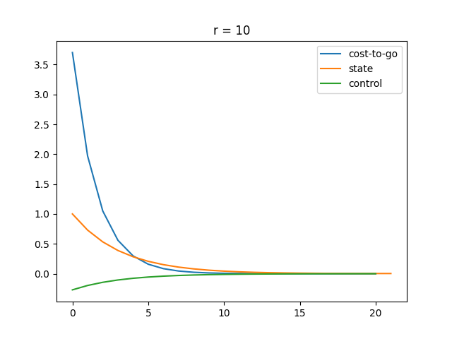
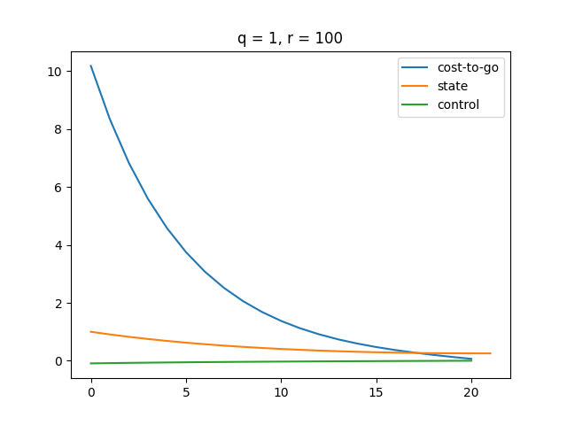
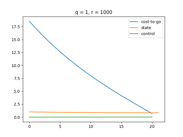
A higher $r$ makes our control more expensive, which results in a smaller magnitude of control. Therefore, we see a smoother state change and cost change. Also, it turns out that our cost function converges slower as $r$ gets bigger.

LQR vs MPC

I'm not able to reach the destination exactly. I got $x_{N} = 0.11034658148808552$, which is close to 0, but not exactly 0. This is because the cost function is designed to measure the deviations of the state and control signals from their desired values, and it always assigns a non-zero cost to these deviations, no matter how small they are. As a result, even if the state and control signals converge to their desired values and the system is perfectly controlled, there will still be a non-zero cost associated with the deviations from the desired values.

Therefore, the goal of the LQR controller is not to achieve zero cost, but rather to minimize the cost function as much as possible, given the system dynamics and the design specifications. The optimal control input is the one that minimizes the cost function over the finite or infinite time horizon, subject to the constraints imposed by the system dynamics and the control design.

An MPC Solution

import matplotlib.pyplot as plt
import cvxpy as cp

if __name__ == '__main__':
    a = 1
    b = 1
    q = 1
    qf = q
    r = 50
    N = 20
    x0 = 1

    x = cp.Variable(N + 1)
    u = cp.Variable(N)

    cost = 0
    constr = []
    T = N

    cost += q * cp.sum_squares(x) + r * cp.sum_squares(u) + qf * x[N] ** 2
    constr += [x[0] == x0]
    constr += [x[N] == 0]
    for t in range(T):
        constr += [x[t + 1] == a * x[t] + b * u[t]]

    prob = cp.Problem(cp.Minimize(cost), constr)

    prob.solve()
    cost = []
    for t in range(N):
        c = q * cp.sum_squares(x[t:]) + r * \
            cp.sum_squares(u[t:]) + qf * x[N] ** 2
        cost.append(c.value)

    # Plot them
    plt.title("q = " + str(q) + ", r = " + str(r))
    plt.plot(range(N), cost, label="cost-to-go")
    plt.plot(range(N + 1), x.value, label="state")
    plt.plot(range(N), u.value, label="control")
    plt.legend()
    plt.show()

Comparison

LQR	MPC
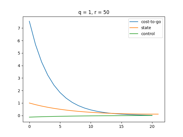There's a small gap between any of the two curves at the end of the time step.	All three curves converge at the last time step, all having a value of $0$.

Trajectory Following Problem

$$\begin{aligned} J_t^*\left(x_t, u_t\right) & =\min _{u_t}\left\{q x_t^2+r u_t^2+J_{t+1}^*\left(x_{t+1}\right)\right\} \\ & =\min _{u_t}\left\{q x_t^2+r u_t^2+p_{t+1} (x_{t+1}-x_{t+1}^*)^2\right\} . \\ & =\min _{u_t}\left\{q x_t^2+r u_t^2+p_{t+1} a^2 (x_t-x_t^*)^2+2 p_{t+1} a b (x_t-x_t^*) u_t+p_{t+1} b^2 u_t^2\right\} \end{aligned}$$

We apply first-order optimality condition $\frac{d J_t^*}{d u_t}=0$

$$\begin{aligned} 2 r u_t+2 p_{t+1} a b (x_t-x_t^*)+2 p_{t+1} b^2 u_t & =0 \\ u_t^* & =-\frac{p_{t+1} a b (x_t-x_t^*)}{r+p_{t+1} b^2}=-k_t (x_t-x_t^*) \\ k_t & =\frac{p_{t+1} a b}{r+p_{t+1} b^2} \end{aligned}$$

$$\begin{aligned} J_t^*\left(x_t\right) & = q (x_t-x_t^*)^2+r\left(-k_t (x_t-x_t^*)\right)^2+p_{t+1} a^2 (x_t-x_t^*)^2 \\ &\quad +2 p_{t+1} a b (x_t-x_t^*)\left(-k_t (x_t-x_t^*)\right) +p_{t+1} b^2\left(-k_t (x_t-x_t^*)\right)^2 \\ &=\left(q+r k_t^2+p_{t+1} a^2-2 p_{t+1} a b k_t+p_{t+1} b^2 k_t^2\right) (x_t-x_t^*)^2 \\ &= p_t (x_t-x_t^*)^2 \\ & \Rightarrow p_t =q+r k_t^2+p_{t+1} a^2-2 p_{t+1} a b k_t+p_{t+1} b^2 k_t^2 \end{aligned}$$

note

This is nothing but changing the $x_t$ to $x_t-x_t^*$.

Plot

Performance

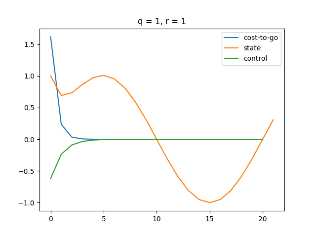
The tracking performance is insanely well. We can see the state function start to behave like a $\sin()$ function around $t = 5$ and cost and control both approach $0$ as well.

Pros and Cons

In LQR, the control law is

• Globally optimal (no approximations involved)
• State feedback (w/o re-optimizing anything)
• Really easy to implement with limited computing (the main reason for its popularity in robotics)

But,

• Limited in its scope
  • No constraints
  • Linear dynamics
  • Quadratic cost function